2. Tumor spatial autocorrelation and clinical prognosis
Lauren Hsu1
Source:vignettes/moran_clinical.Rmd
moran_clinical.RmdIntroduction
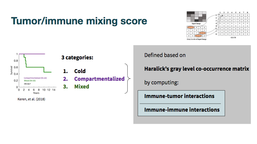
In this vignette, I examine the Moran’s index and its associations to the clinically prognostic tumor categories set forth by the authors in A Structured Tumor-Immune Microenvironment in Triple Negative Breast Cancer Revealed by Multiplexed Ion Beam Imaging.
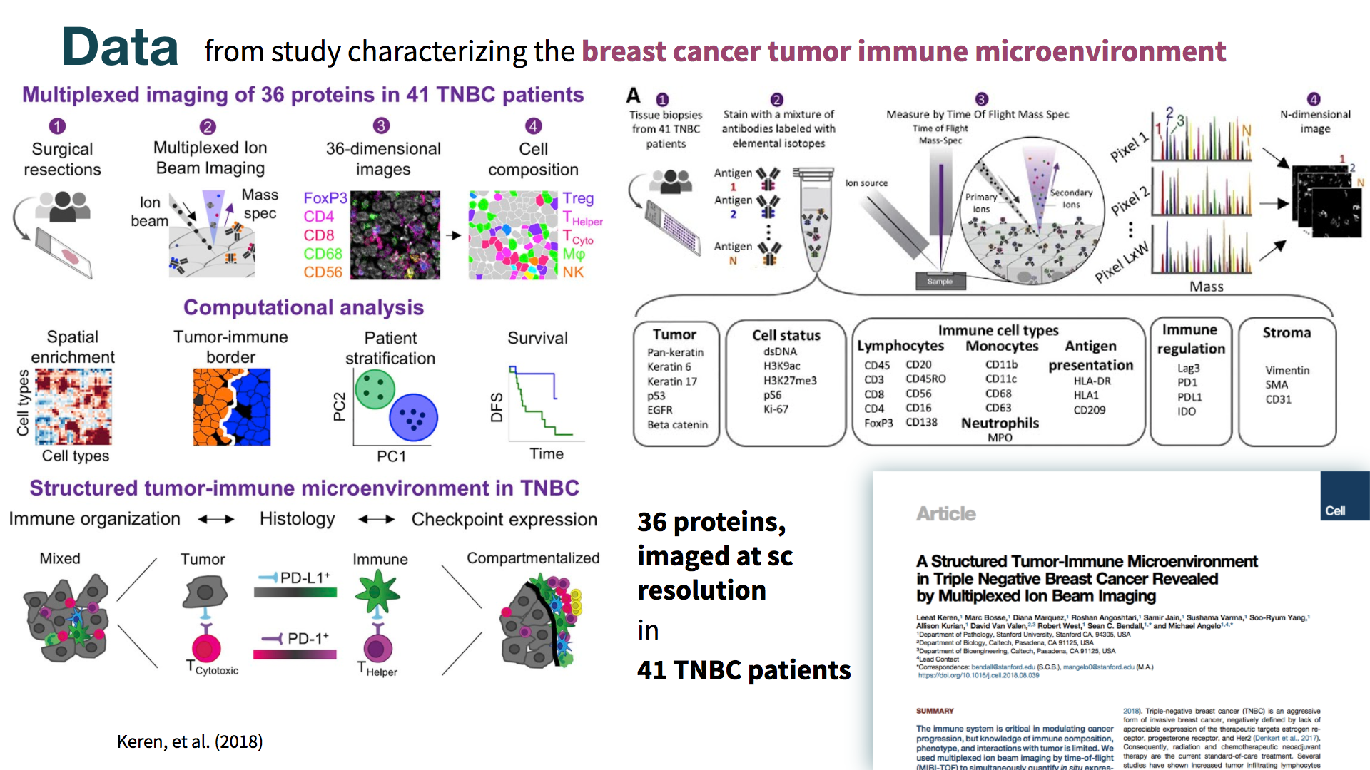
Visit the BIRSBiointegration Hackathon page to read more about MIBI-TOF.
Loading data
resMoranTest.csv is the output from running compute_morans.R on the mibiTOF segmented image files, downloadable here: https://www.angelolab.com/mibi-data
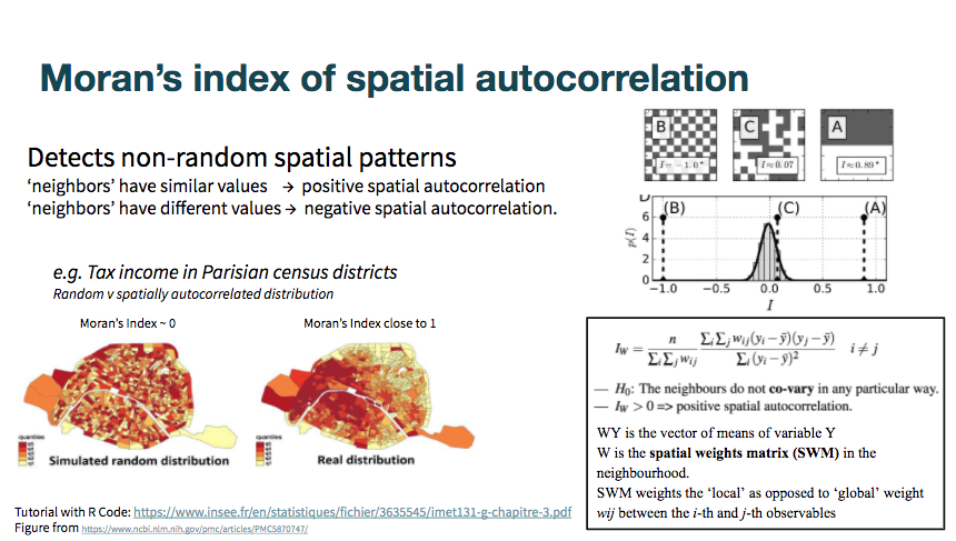
A key component used in computing Moran’s I is the spatial weighting matrix (SWM). This can be formed from any number of ways, including by various distance metrics (e.g., Euclidean), by graphs, or any other ways of defining proximity in space.
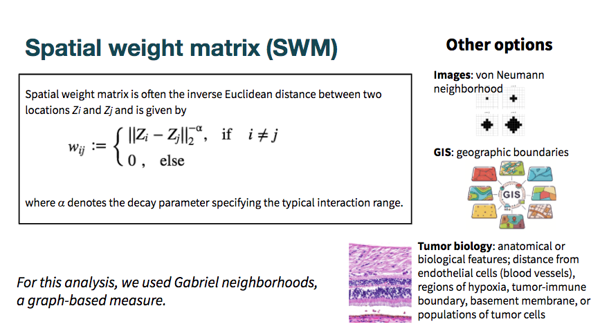
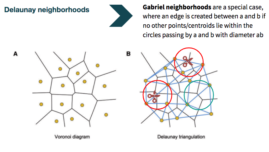
We used SWM defined by Gabriel neighborhoods, which is a special case of a Delaunay graph (constructed from Voronoi tesselation). Delaunay graphs are constructed by drawing edges between all nodes with shared Voronoi faces (light blue edges and yellow nodes on the bottom right below). To then transform the graph into a Gabriel graph, edges are pruned if there are other points that lie within the smallest circle passing through those two points (e.g., in the red circles below), and edges are kept if not (e.g., in the green circle below).
patient_class.csv is included in the download from the link above. For each sample it contains the tumor classification as defined in the paper:
Moran plots
Computing p-values for 3-way ANOVA test of significance for Moran’s I on the dummy variables (cell type flags) and each protein expression level.
moran_aov <- moran[,-1]
moran_aov$class <- as.factor(moran_aov$class)

feats <- colnames(moran_aov)[-42]

pvals <- data.frame(matrix(NA, ncol = 2, nrow = length(feats)))
colnames(pvals) <- c('feat','aov_pval')
rownames(pvals) <- feats

for (feat in feats){
  pvals[feat,] <- c(feat,summary(aov(moran_aov[,feat] ~ moran_aov[,'class']))[[1]][['Pr(>F)']][1])
}

pvals$aov_pval <- as.numeric(pvals$aov_pval)

pvals <- pvals[order(pvals$aov_pval),]
Individual ANOVA tests: (3 sets; for each, the other 2 groups are coded together as “other”)
moran_aov_sep <- moran[,-1]
moran_aov_sep$class_cold <- as.factor(plyr::mapvalues(moran_aov_sep$class,
                               from = c('mixed','compartment','cold'),
                               to = c('other','other','cold')))
moran_aov_sep$class_mixed <- as.factor(plyr::mapvalues(moran_aov_sep$class,
                               from = c('mixed','compartment','cold'),
                               to = c('mixed','other','other')))
moran_aov_sep$class_comp <- as.factor(plyr::mapvalues(moran_aov_sep$class,
                               from = c('mixed','compartment','cold'),
                               to = c('other','compartment','other')))

feats <- colnames(moran_aov_sep)[c(-45:-42)]

pvals_sep <- data.frame(matrix(NA, ncol = 4, nrow = length(feats)))
colnames(pvals_sep) <- c('feat','test_cold','test_mixed','test_comp')
rownames(pvals_sep) <- feats

for (feat in feats){
  pvals_sep[feat,] <- c(feat,
                        summary(aov(moran_aov_sep[,feat] ~ moran_aov_sep[,'class_cold']))[[1]][['Pr(>F)']][1],
                        summary(aov(moran_aov_sep[,feat] ~ moran_aov_sep[,'class_mixed']))[[1]][['Pr(>F)']][1],
                        summary(aov(moran_aov_sep[,feat] ~ moran_aov_sep[,'class_comp']))[[1]][['Pr(>F)']][1])
}

pvals_sep[rownames(pvals),]
##                      feat           test_cold           test_mixed
## tumorYN           tumorYN  0.0341255910828547  0.00138488568677017
## CD45                 CD45 0.00926810561241914   0.0172991570917716
## CD45RO             CD45RO   0.153768342349517 0.000847841247869497
## CD11c               CD11c  0.0359573772907523   0.0106009334311595
## CD4                   CD4   0.272629983491842 0.000990523269478657
## Beta.catenin Beta.catenin   0.441713353948455 0.000633966876022113
## CSF.1R             CSF.1R  0.0260297339236067   0.0734092694590058
## CD3                   CD3   0.231378899113043  0.00606288943242979
## Pan.Keratin   Pan.Keratin   0.280025985796279  0.00733873289803587
## CD8                   CD8 0.00881687281664925       0.247950391012
## H3K9ac             H3K9ac 0.00768400905209691  0.00332980957925492
## HLA.DR             HLA.DR   0.721556225584227  0.00268378125355884
## PD.L1               PD.L1 0.00189108015255096    0.973256320059549
## PD1                   PD1   0.396163920509005    0.010541639052546
## Keratin6         Keratin6   0.191068629524341   0.0324436596735067
## CD11b               CD11b  0.0507890928320497    0.208960309971905
## Vimentin         Vimentin   0.157054785990441  0.00337777238568537
## CD20                 CD20   0.343906470528576   0.0202168392251092
## cellSize         cellSize   0.495024045383168   0.0224414424296167
## CD16                 CD16  0.0203026161959533    0.643303061732047
## CD163               CD163   0.774417327487516   0.0200755355846754
## CD138               CD138  0.0321922296600026   0.0670285683964105
## HLA_Class_1   HLA_Class_1   0.575185456376524   0.0152914905787428
## phospho.S6     phospho.S6   0.356008033837109   0.0204491896010629
## H3K27me3         H3K27me3   0.573476548037953   0.0252502986964708
## Keratin17       Keratin17    0.48333491261473   0.0264463023616048
## p53                   p53    0.02920027513594    0.621112186580165
## CD209               CD209   0.075665916309574    0.594684205683068
## OX40                 OX40   0.407556206139695    0.122410375469582
## CD31                 CD31   0.596672323390244   0.0946218569210861
## Lag3                 Lag3   0.972418703053599   0.0448862813916235
## B7H3                 B7H3  0.0524360558556027    0.387246616574369
## Ki67                 Ki67   0.928414429412843    0.128460352975178
## MPO                   MPO   0.230393392178348    0.587012118460728
## IDO                   IDO   0.980359448027047    0.177751252998018
## CD68                 CD68   0.200304931399538    0.799693019882516
## SMA                   SMA   0.381927436545846     0.27226501530817
## FoxP3               FoxP3   0.293454923929008    0.450073122721021
## CD63                 CD63   0.899182243125353    0.319317727598852
## CD56                 CD56   0.325289880739089    0.626169875408483
## EGFR                 EGFR   0.761672949319811    0.851555474947503
##                         test_comp
## tumorYN      5.01078563984276e-08
## CD45         2.97989056262974e-06
## CD45RO       1.13364321116951e-06
## CD11c        8.49490976222607e-06
## CD4          8.18904341534503e-06
## Beta.catenin 1.84599969895042e-05
## CSF.1R       0.000411883978663573
## CD3          0.000110353888557948
## Pan.Keratin   0.00022813542098335
## CD8           0.00252248271314348
## H3K9ac          0.232016396221856
## HLA.DR       0.000619848715663221
## PD.L1          0.0445801939992952
## PD1           0.00083481369919345
## Keratin6      0.00124082021354464
## CD11b         0.00749451883529667
## Vimentin       0.0473951787483856
## CD20          0.00352866245988334
## cellSize      0.00379811596789498
## CD16           0.0448972617394975
## CD163          0.0109454363422921
## CD138           0.627399123706833
## HLA_Class_1    0.0356832322421822
## phospho.S6     0.0822829730944162
## H3K27me3       0.0560420017774816
## Keratin17      0.0726084698341079
## p53             0.373008733951914
## CD209           0.105807280220194
## OX40           0.0338333250955215
## CD31           0.0348130551865471
## Lag3           0.0408842537259478
## B7H3            0.458033396966791
## Ki67           0.0979176465990246
## MPO             0.173574551750504
## IDO             0.166727117095437
## CD68            0.567440678482007
## SMA             0.579516983961658
## FoxP3           0.867616415535372
## CD63            0.344490529642514
## CD56            0.980073086236272
## EGFR            0.693654383426714
Visualizing Moran’s I across groups
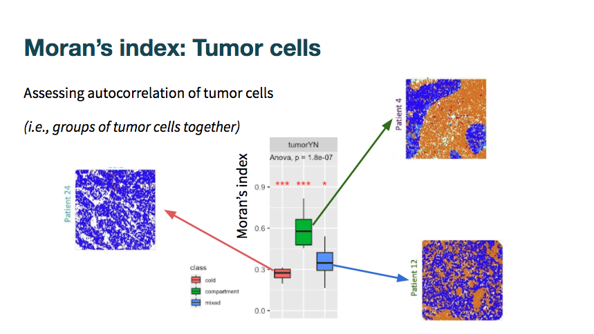
Comparing Moran’s I scores across the clinical prognosis categories on the tumor cell dummy variable:
(Moran’s I is computed where the measurement in each cell is 1 or 0, for whether is is or is not a tumor cell, providing a measure of spatial autocorrelation of tumor cells within the sample.)
ggplot(moran, aes(x=class, y=tumorYN)) +
  geom_boxplot(aes(fill = class))
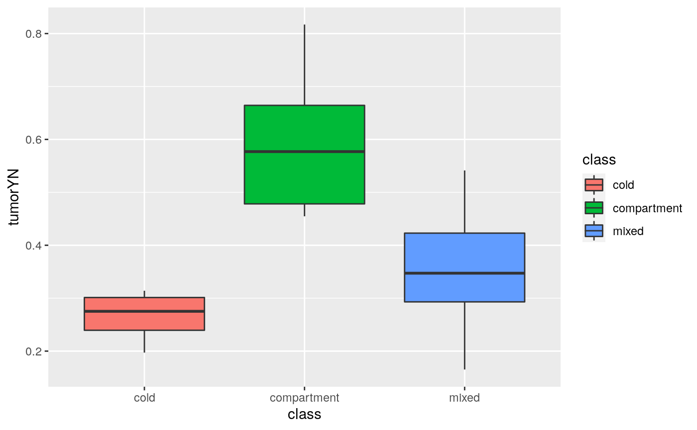
Here, we can see the differences when visualized alongsidem images of the tumors (tumor images as published by Keren et al. 2018)
Comparing all attributes:
(Each panel corresponds to a given attribute, mostly proteins, and shows the differences in spatial autocorrelation, as quantified with Moran’s I, across the clinical groups. Panels are sorted by p-value of 3 way anova, and include *s to indicate their significance level in the “each vs rest” ANOVA tests.)
moran_melt <- melt(moran,id.vars = c('sample','class'))
moran_melt$variable <- factor(moran_melt$variable, levels = rownames(pvals)) # sort panels by 3way anova pval

mm <- ggplot(moran_melt, aes(x=class, y=value)) +
  geom_boxplot(aes(fill = class)) + facet_wrap(. ~ variable, nrow = 3) +
  stat_compare_means(method = "anova", label.y = 1.1, size = 3) +      # Add global p-value
  stat_compare_means(label = "p.signif", method = "t.test",
                     ref.group = ".all.", hide.ns = TRUE, color = 'red', size = 3) +
  theme(axis.text.x=element_blank(),
        axis.ticks.x=element_blank())

Defining some proteins that may be interesting to consider together, due to related cell types / function:
immune_subset <-c('CD45','CD45RO', 'CD3','CD8', 'CD16','CD163','HLA.DR')
immune_subset2 <-c('CD45','CD45RO', 'CD3','CD8', 'CD16','CD163','HLA.DR', 'CD11c')
monocyte_subset <- c('CD11b','CD11c','CD68','CD63')
im_reg_subset <- c('PD1','PD.L1')
tum_subset <- c('tumorYN', 'Beta.catenin', 'Pan.Keratin', 'Keratin6', 'EGFR', 'p53')
lymphocytes <- c('CD45','CD3','CD8','CD4','CD20','CD45RO','CD56','CD16','CD138')
antigen_prez <- c('HLA.DR','HLA_Class_1', 'CD209')
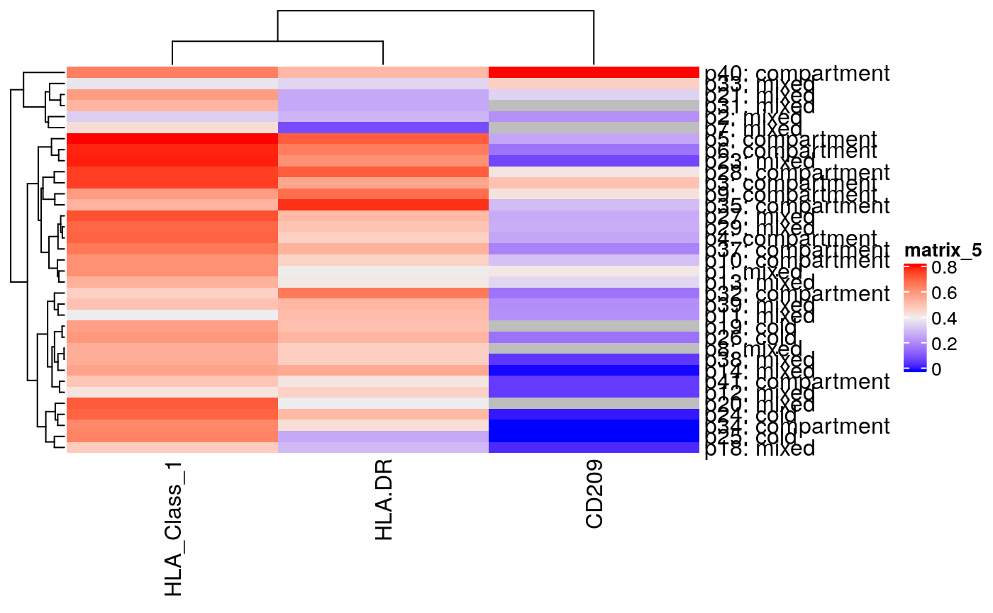
Examining a few of the protein subsets
for(cur_sub in list(immune_subset, monocyte_subset, tum_subset, lymphocytes, antigen_prez)){
  moran_melt <- melt(moran[,c('sample','class',cur_sub)],id.vars = c('sample','class'))
  moran_melt$variable <- factor(moran_melt$variable,
                                levels = rownames(pvals)[rownames(pvals) %in% cur_sub])
  # sort panels by 3way anova pval

  ggplot(moran_melt, aes(x=class, y=value)) +
    geom_boxplot(aes(fill = class)) + facet_wrap(. ~ variable, ncol = 5) +
    stat_compare_means(method = "anova", label.y = 1.1, size = 3) +      # Add global p-value
    stat_compare_means(label = "p.signif", method = "t.test",
                       ref.group = ".all.", hide.ns = TRUE, color = 'red', size = 5) +
    theme(axis.text.x=element_blank(),
          axis.ticks.x=element_blank())
  moranHM <- moran[,-c(1,43)]
  moranHM <- moranHM[,cur_sub]
  rownames(moranHM) <- paste(moran$sample,moran$class,sep = ': ')
  show(ComplexHeatmap::Heatmap(moranHM))
}
## Warning: The input is a data frame, convert it to the matrix.

## Warning: The input is a data frame, convert it to the matrix.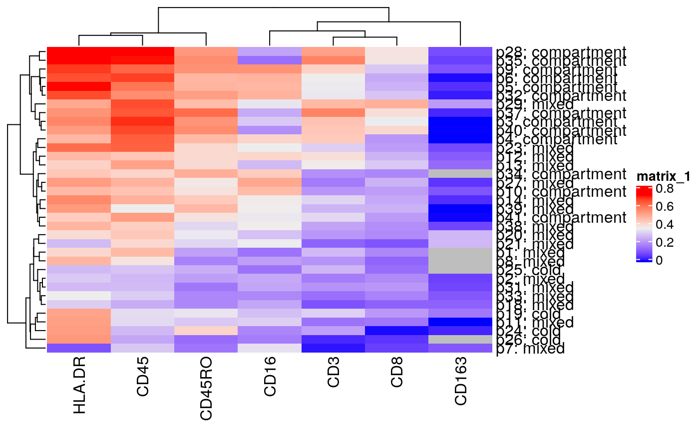
## Warning: The input is a data frame, convert it to the matrix.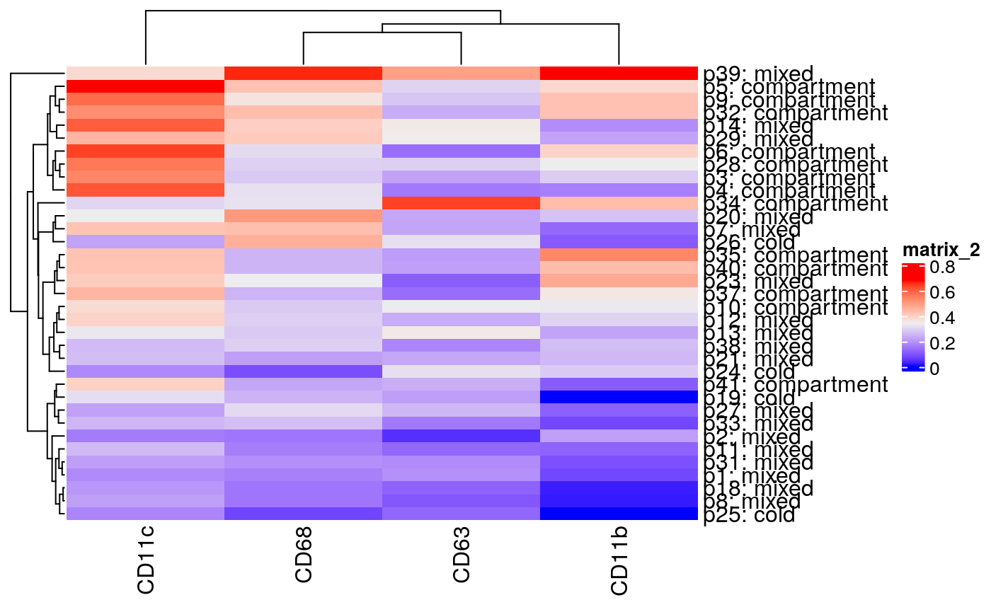
## Warning: The input is a data frame, convert it to the matrix.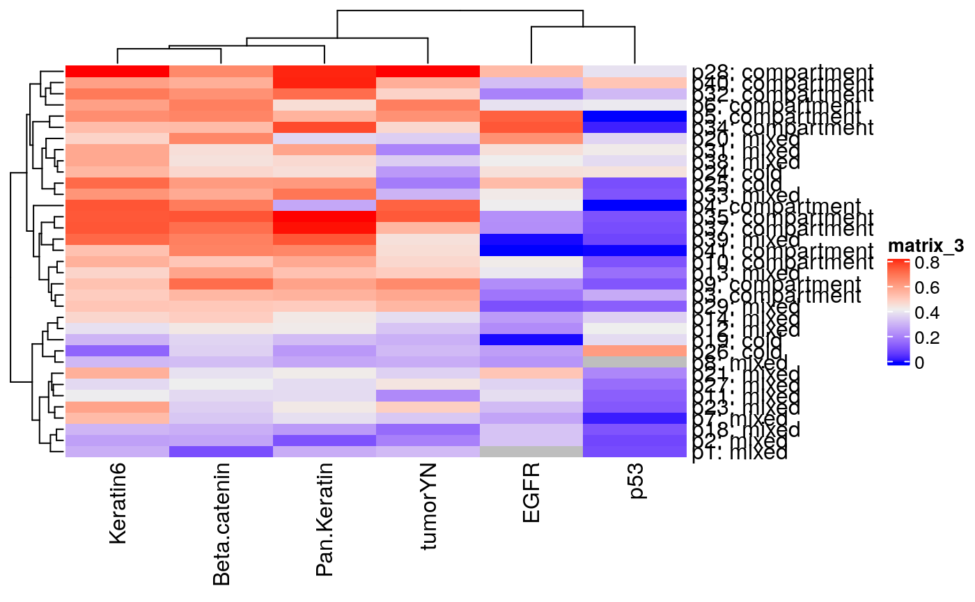
## Warning: The input is a data frame, convert it to the matrix.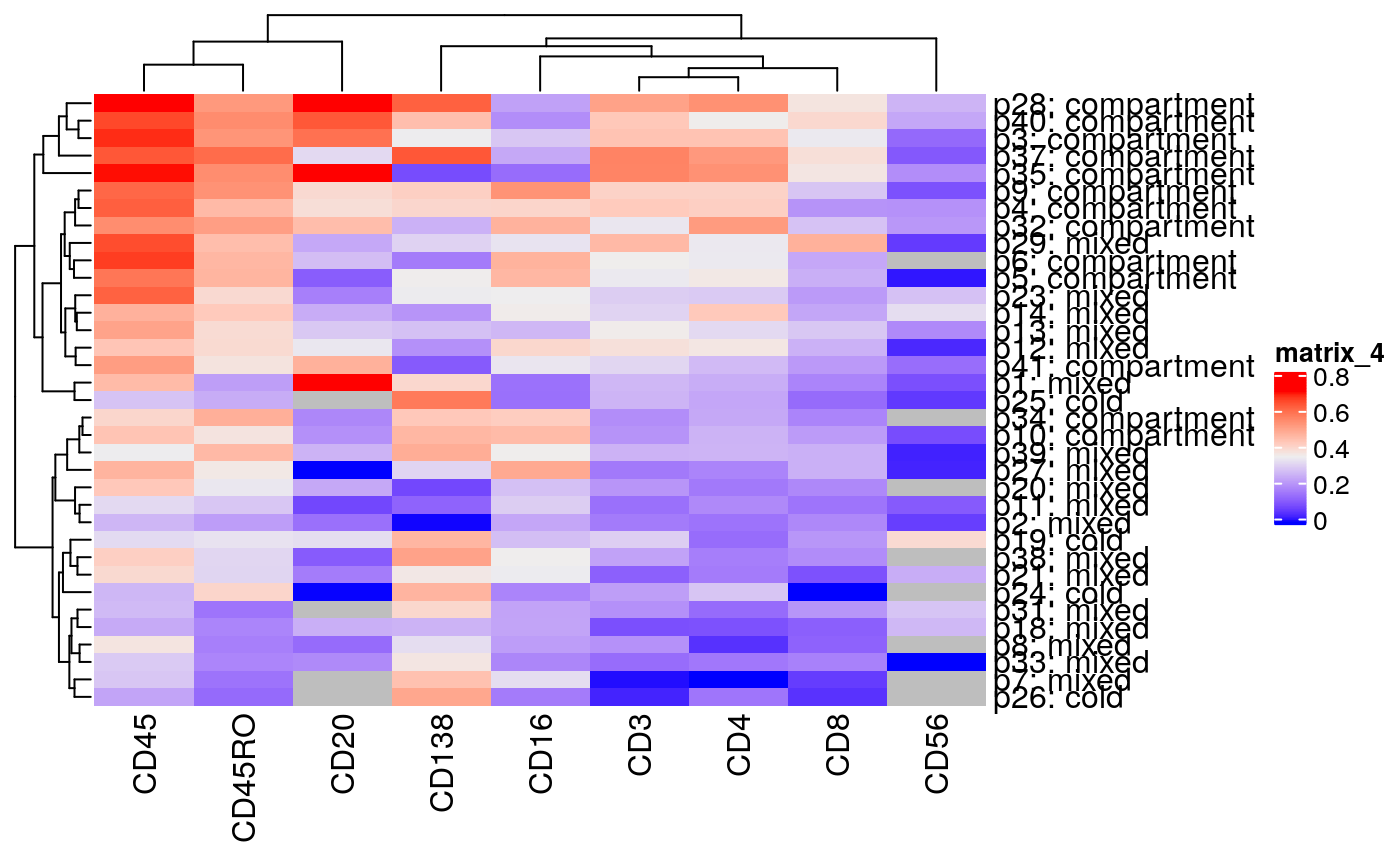
Additional visualizations
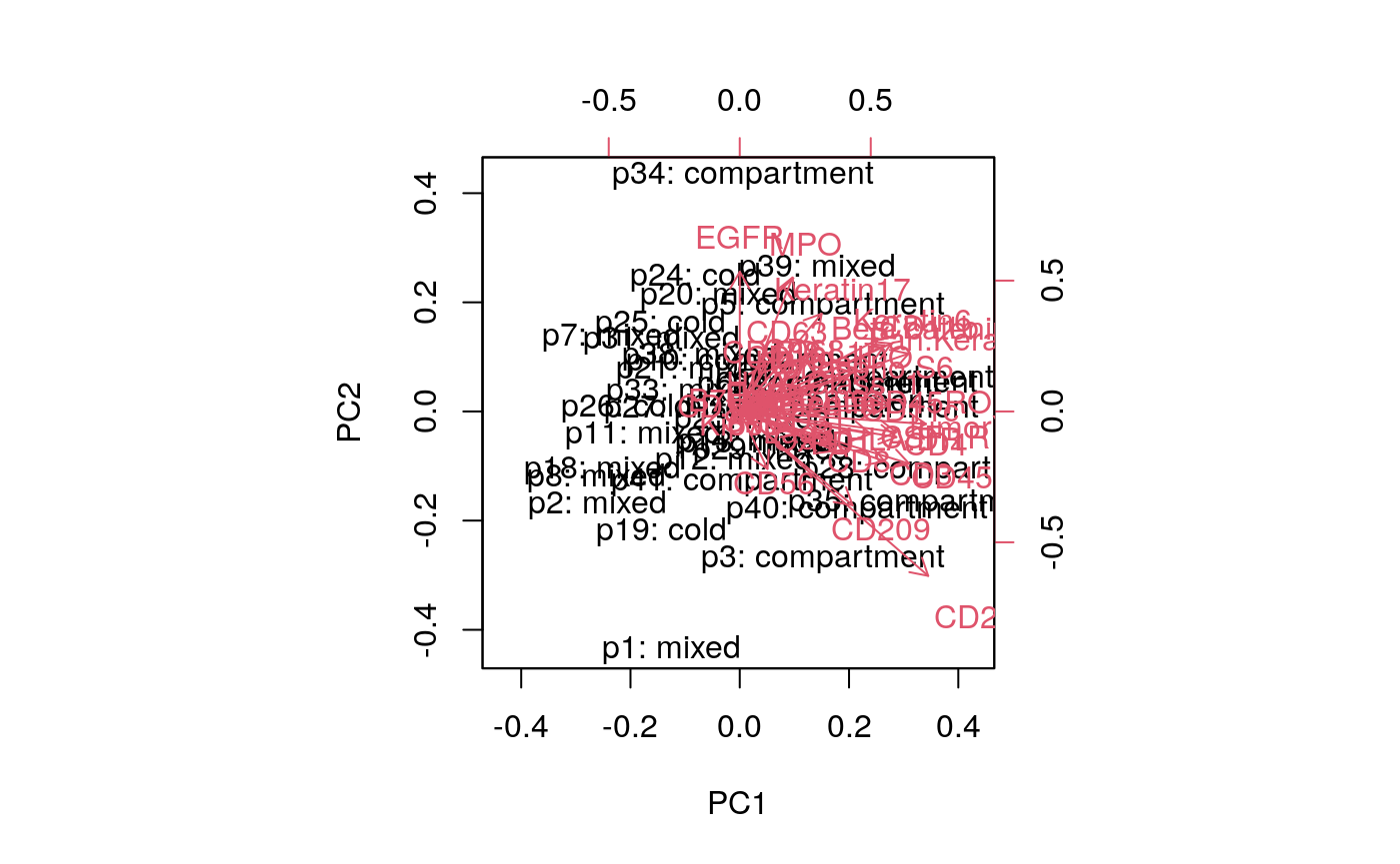
Biplot: samples labeled by tumor class and proteins
moran_bip <- corral::na2zero(moran_aov[,-42])
rownames(moran_bip) <- paste(moran$sample,moran$class,sep = ': ')
prc_moran <- prcomp(moran_bip)
biplot(prc_moran)
Heatmap of the Moran’s I values per protein, per sample.
moranHM <- moran[,-c(1,43)]
rownames(moranHM) <- paste(moran$sample,moran$class,sep = ': ')
ComplexHeatmap::Heatmap(moranHM)
## Warning: The input is a data frame, convert it to the matrix.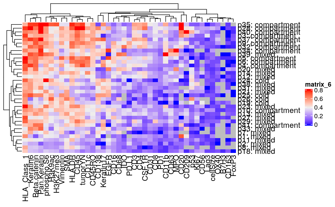
Harvard School of Public Health↩︎